Observational Routines
The following functions provide additional mock observing features for use with the coronagraph model.
-
coronagraph.observe.get_earth_reflect_spectrum()¶ Get the geometric albedo spectrum of the Earth around the Sun. This was produced by Tyler Robinson using the VPL Earth Model (Robinson et al., 2011)
- Returns
lamhr (numpy.ndarray)
Ahr (numpy.ndarray)
fstar (numpy.ndarray)
-
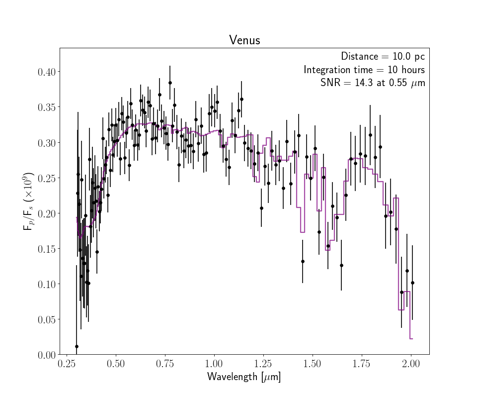
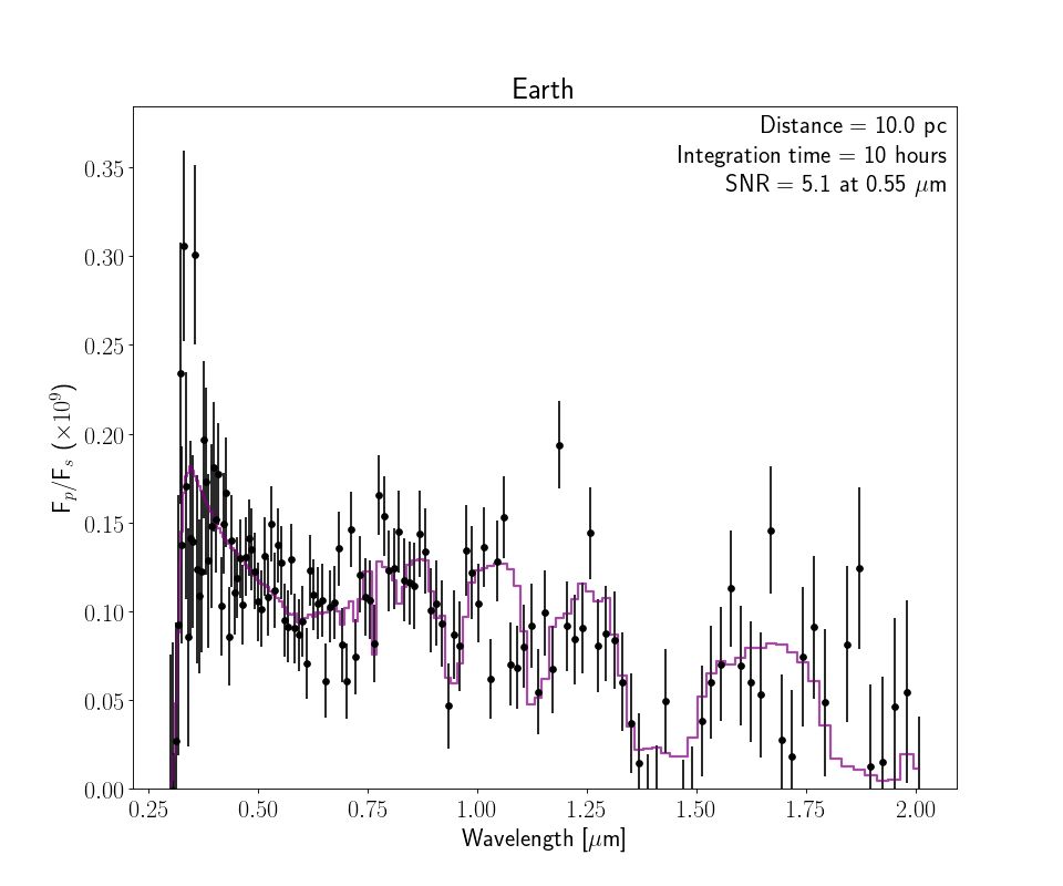
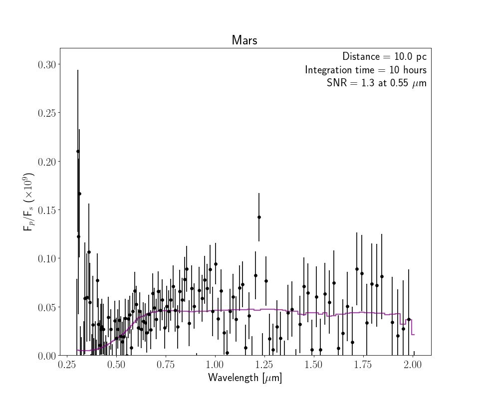
coronagraph.observe.planetzoo_observation(name='earth', telescope=<coronagraph.teleplanstar.Telescope object>, planet=<coronagraph.teleplanstar.Planet object>, itime=10.0, planetdir='/home/docs/checkouts/readthedocs.org/user_builds/coronagraph/conda/latest/lib/python3.5/site-packages/coronagraph-1.0-py3.5.egg/coronagraph/planets/', plot=False, savedata=False, saveplot=False, ref_lam=0.55, THERMAL=False)¶ Observe the Solar System planets as if they were exoplanets.
- Parameters
name (str (optional)) –
- Name of the planet. Possibilities include:
”venus”, “earth”, “archean”, “mars”, “earlymars”, “hazyarchean”, “earlyvenus”, “jupiter”, “saturn”, “uranus”, “neptune”
telescope (Telescope (optional)) – Telescope object to be used for observation
planet (Planet (optional)) – Planet object to be used for observation
itime (float (optional)) – Integration time (hours)
planetdir (str) – Location of planets/ directory
plot (bool (optional)) – Make plot flag
savedata (bool (optional)) – Save output as data file
saveplot (bool (optional)) – Save plot as PDF
ref_lam (float (optional)) – Wavelength at which SNR is computed
- Returns
lam (array) – Observed wavelength array (microns)
spec (array) – Observed reflectivity spectrum
sig (array) – Observed 1-sigma error bars on spectrum
Example
>>> from coronagraph.observe import planetzoo_observation
>>> lam, spec, sig = planetzoo_observation(name = "venus", plot = True)
>>> lam, spec, sig = planetzoo_observation(name = "earth", plot = True)
>>> lam, spec, sig = planetzoo_observation(name = "mars", plot = True)
-
coronagraph.observe.generate_observation(wlhr, Ahr, solhr, itime, telescope, planet, star, ref_lam=0.55, tag='', plot=True, saveplot=False, savedata=False, THERMAL=False, wantsnr=10)¶ (Depreciated) Generic wrapper function for count_rates.
- Parameters
wlhr (float) – Wavelength array (microns)
Ahr (float) – Geometric albedo spectrum array
itime (float) – Integration time (hours)
telescope (Telescope) – Telescope object
planet (Planet) – Planet object
star (Star) – Star object
tag (string) – ID for output files
plot (boolean) – Set to True to make plot
saveplot (boolean) – Set to True to save the plot as a PDF
savedata (boolean) – Set to True to save data file of observation
- Returns
lam (array) – Wavelength grid for observed spectrum
dlam (array) – Wavelength grid widths for observed spectrum
A (array) – Low res albedo spectrum
spec (array) – Observed albedo spectrum
sig (array) – One sigma errorbars on albedo spectrum
SNR (array) – SNR in each spectral element
Note
If saveplot=True then plot will be saved If savedata=True then data will be saved
-
coronagraph.observe.plot_coronagraph_spectrum(wl, ofrat, sig, itime, d, ref_lam, SNR, truth=None, xlim=None, ylim=None, title='', save=False, tag='')¶ Plot synthetic data from the coronagraph model
- Parameters
wl (array-like) – Wavelength grid [microns]
ofrat (array-like) – Observed contrast ratio (with noise applied)
sig (array-like) – One-sigma errors on
ofratitime (float) – Integration time for calculated observation [hours]
d (float) – Distance to system [pc]
ref_lam (float) – Reference wavelength [microns]
SNR (array) – Signal-to-noise
truth (array-like (optional)) – True contrast ratio
xlim (list (optional)) – Plot x-axis limits
ylim (list (optional)) – Plot y-axis limits
title (str (optional)) – Plot title and saved plot name
save (bool (optional)) – Set to save plot
tag (str (optional)) – String to append to saved file
- Returns
fig (matplotlib.Figure)
ax (matplotlib.Axis)
Note
Only returns
fig, axifsave = False
-
coronagraph.observe.process_noise(Dt, Cratio, cp, cb)¶ Computes SNR, noised data, and error on noised data.
- Parameters
Dt (float) – Telescope integration time in seconds
Cratio (array) – Planet/Star flux ratio in each spectral bin
cp (array) – Planet Photon count rate in each spectral bin
cb (array) – Background Photon count rate in each spectral bin
- Returns
cont (array) – Noised Planet/Star flux ratio in each spectral bin
sigma (array) – One-sigma errors on flux ratio in each spectral bin
SNR (array) – Signal-to-noise ratio in each spectral bin
-
coronagraph.observe.random_draw(val, sig)¶ Draw fake data points from model
valwith errorssig
-
coronagraph.observe.interp_cont_over_band(lam, cp, icont, iband)¶ Interpolate the continuum of a spectrum over a masked absorption or emission band.
- Parameters
lam (array) – Wavelength grid (abscissa)
cp (array) – Planet photon count rates or any spectrum
icont (list) – Indicies of continuum (neighboring points)
iband (list) – Indicies of spectral feature (the band)
- Returns
ccont – Continuum planet photon count rates across spectral feature, where len(ccont) == len(iband)
- Return type
list
-
coronagraph.observe.exptime_band(cp, ccont, cb, iband, SNR=5.0)¶ Calculate the exposure time necessary to get a given S/N on a molecular band following Eqn 7 from Robinson et al. (2016),
\({\rm{S}}/{{\rm{N}}}_{\mathrm{band}}=\displaystyle \frac{{\displaystyle \sum }_{j}\;{c}_{{\rm{cont,}}j}-{c}_{{\rm{p,}}j}}{\sqrt{{\displaystyle \sum }_{j}\;{c}_{{\rm{p,}}j}+2{c}_{{\rm{b,}}j}}}\;\Delta {t}_{\mathrm{exp}}^{1/2}\)
where the sum is over all spectral elements (denoted by subscript “j”) within the molecular band.
- Parameters
cp – Planet count rate
ccont – Continuum count rate
cb – Background count rate
iband – Indicies of molecular band
SNR – Desired signal-to-noise ratio on molecular band
- Returns
texp – Telescope exposure time [hrs]
- Return type
float
-
coronagraph.observe.plot_interactive_band(lam, Cratio, cp, cb, itime=None, SNR=5.0)¶ Makes an interactive spectrum plot for the user to identify all observed spectral points that make up a molecular band. Once the plot is active, press ‘c’ then select neighboring points in the Continuum, press ‘b’ then select all points in the Band, then press ‘d’ to perform the calculation.
- Parameters
lam (array) – Wavelength grid
Cratio (array) – Planet-to-star flux contrast ratio
cp (array) – Planetary photon count rate
cb (array) – Background photon count rate
itime (float (optional)) – Fiducial exposure time for which to calculate the SNR
SNR (float (optional)) – Fiducial SNR for which to calculate the exposure time